Let us suppose that your data is in the A column. Copy this formula in the B column
=COUNTIF(A$1:A1,A2)=0
This formula will check from A1 to the current cell for any Duplicates. It will return TRUE if no Duplicate is there and FALSE if Duplicate is found as shown here
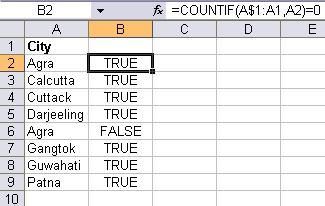
Now you can filter all the FALSE entries and you will get the unique records.
Method 1(a).
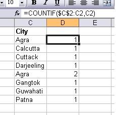
Here is another version of the above formula:
=COUNTIF(A$1:A1,A2)
This will do the same job as above but will return 1 if no Duplicate is there and FALSE if Duplicate is found as shown here
Method 2.
Step 1. Select the column containing data including headings.
Step 2. Go to DATA menu Filter >> Advanced Filter
Step 3. In the Advanced Filter dialog box, make sure that the Filter the list, in place is selected.
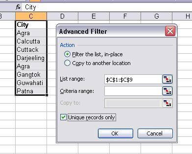
Results: You will see reults like this :Method 1(a).
Here is another version of the above formula:
=COUNTIF(A$1:A1,A2)

Method 2.
This method involves filtering of data. The steps are as follows:
Step 2. Go to DATA menu Filter >> Advanced Filter
Step 3. In the Advanced Filter dialog box, make sure that the Filter the list, in place is selected.
Step 4. Check the Unique records only check box, and then click OK.

You can see that the Duplicate row Row(6) is not shown in the results. You can copy the results and paste them elsewhere.


No comments:
Post a Comment